

Introduction
Introducing a faster, data-fueled marketing mindset
In this day and age, consumers have more choice than ever before. They can easily harness their scrolling abilities to get pretty much whatever they want, whenever they want it. Fueled by the pandemic and a growing demand for digital services and entertainment, competition in the app market has become fiercer than ever before.
Staying a step ahead of the curve is the only way to remain competitive. And predictive modeling enables just that, helping marketers understand consumer behaviors and trends, predicting future actions, and planning their campaigns based on data-driven decisions.
The science of predictive analytics has been around for years, and used by the largest companies in the world to perfect their operations, anticipate supply and demand shifts, foresee global changes, and use historical data to better prepare for future events.
But what is this strange, data science & marketing brainchild, you ask?
Predictive modeling is a form of analysis that leverages machine learning and AI to examine historical campaign data, past user behavior data, and additional transactional data to predict future actions.
Using predictive modeling, marketers can make rapid campaign optimization decisions without having to wait for actual results to come in. For example, a machine learning algorithm has found that users who completed level 10 of a game within the first 24 hours were 80% more likely to make an in-app purchase within the first week.
Armed with this knowledge, marketers can optimize after that event is reached within 24 hours, well before the first week has gone by. If the campaign isn’t performing well, continued investment would be a complete waste of budget. But if it is, quickly doubling down on investment can drive even better results.
What about privacy?
What impact does privacy have on predictive modeling now that there is limited access to user-level data?
It’s a known fact that mobile users have become increasingly sophisticated and knowledgeable over the past few years. With privacy (or lack of) taking center stage, the average app user is no longer in a hurry to provide their data in order to use an app, or even to enjoy a more personalized experience.
But, in 2021, are advertisers really left in the dark when it comes to access to quality data?
The short answer is not necessarily. By combining predictive modeling, SKAdNetwork, aggregated data, and cohort analysis, marketers can make informed decisions even in an IDFA-limited reality.
But where to begin? It’s one thing to measure events, monitor performance, and optimize. It’s another thing entirely to analyze a massive amount of data, as well as develop and apply predictive models that will enable you to make nimble, accurate data-driven decisions.
Well, fear not. We’re here to help you make sense of it all.
In this practical guide – a collaboration between AppsFlyer, digital marketing agency AppAgent, and Incipia, we’ll be exploring how marketers can take their data skills to the next level and gain that coveted competitive edge with predictive modeling.

Predictive modeling: Basic concepts and measurement setup
Why build predictive models in the first place?
There are numerous benefits to predictive modeling in mobile marketing, but we narrowed it down to two key marketing activities:
1. User acquisition
Knowing your typical user behavior and the early milestones that separate users with high potential and users with low potential can be useful on both the acquisition and re-engagement fronts.
For example, if a user needs to generate X dollars by day 3 to make a profit after day 30, and that number comes in under your benchmark, you’ll know that you will need to adjust bids, creatives, targeting or other things in order to improve the cost / quality of your acquired users, or else improve your monetization trends.
If, however, that X comes in over your benchmark, then you can feel confident in raising budgets and bids to gain even more value from your acquired users.
2. Privacy-centric advertising
For years, online advertising’s biggest advantage over traditional advertising was the ability to use significant amounts of measurable performance data to pinpoint its desired target audience.
The more specific your campaigns are – the more you’re likely to drive higher user LTV and efficient budgeting. But what if you could open the gates to a larger sample group and gain immediate insight into their potential value?
Predictive modeling allows you to do exactly that; expand your campaign’s potential audience. By creating different behavioral characteristic clusters, your audience can then be segmented not by their identity, but their interaction with your campaign in its earliest stages.
What should I measure?
To understand what you need to measure in order to get your predictions right, let’s explore which data points are useful and which are not:
Metrics
Just like the square and rectangle relationship: all metrics are data points, but not all metrics are key performance indicators (KPIs). Metrics are easier to calculate and mature much quicker than KPIs, which tend to involve complex formulas.
Note that with Apple’s SKAdNetwork, the following metrics can still be measured, but with a lesser level of accuracy. More on this in chapter 5.
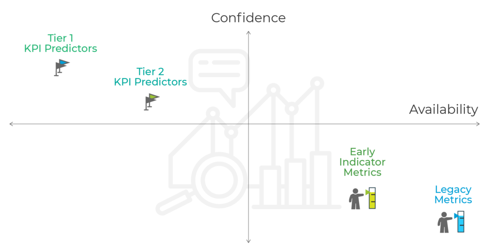
1) Legacy metrics are usually identified with low confidence in predicting profit, but have the fastest availability:
- Click to install (CTI) – the direct conversion between the two strongest touchpoints on a pre-install user journey, CTI is both socially and technically critical, as lower rates might indicate a non-relevant audience, ineffective creatives, or slow loading time prior to an install being completed.
Formula: Number of installs / Number of ad clicks
- Click-through-rate (CTR) – the ratio between a click on a given ad to the total number of views. Higher in the funnel, CTR has limited value informing other overall marketing goals, but can directly reflect the effectiveness of a campaign’s creative based on its recieved clicks.
Formula: number of clicks / Number of ad views.
Required data points: impressions, clicks, attributed installs
2) Early indicator metrics are usually identified with medium confidence in predicting profit and fast availability.
In the age of down-funnel focus, an install is no longer a sufficient KPI. That said, the following metrics, while not useful for use in profit predictions, are still useful as early indicators informing marketers on the likelihood of their campaigns to turn a profit.
Examples include:
- Cost per install (CPI) – Focusing on paid installs rather than organic ones, CPI measures your UA costs in response to viewing an ad.
Formula: Ad spend / Total # of Installs directly tied to ad campaign
- Retention rate – The number of returning users after a given time period.
Calculation: [(CE – CN) / CS)] X 100
CE = number of users at the end of the period
CN = number of new users acquired during the period
CS = number of users at the start of the period
Required data points: cost, attributed installs, app opens, (retention report)
With the exception of retention rate, metrics tend to be tied to a marketing model rather than your business model, and as such, are not useful for determining whether your acquired users will turn a profit for your business.
If you pay $100 per click or per install, chances are that you’re not going to turn a profit. If your CTR is .05%, it’s likely that the auction mechanics will force you to pay a high rate per install, leaving you once again with less margin to turn a profit.
Metrics fail to support predictions when you try to calibrate your confidence range to a finer accuracy, for example – when the line of profitability is within a $2 to $6 CPI range.
KPIs
It is important to sub-divide the common KPIs into two buckets:
1) Tier 2 KPI confident predictors – defined by a medium-high confidence in predicting profit and slow availability:
These are useful to serve as early benchmarks of profit, offering more confidence than leading indicators (metrics), tier 2 KPIs take more time to mature, and also offer less confidence than tier 1 KPIs.
* Note that with Apple’s SKAdNetwork, the following KPIs cannot be measured together.
- Customer acquisition cost per paying user
- Cost or conversion of key actions – e.g. ratio of games in first day played, or ratio of content views during first session
- Time-based cost or conversion of key actions (e.g. cost per number of games played on day one or cost per content view during first session)
- Cost per day X for retained user: Total spend per day X the number of retained users on that day.
- Vertical specific in-app events – e.g. tutorial completion, completing level 5 on day 1 (gaming), number of product pages viewed on 1st session, number of sessions in 24 hours (shopping), etc.
Required data points: cost, attributed installs, app opens (retention report), in-app events configured and measured, session data (time stamps, features used etc.)
For most business models, these KPIs cannot serve as confident predictors because, while they do account for cost and events commonly correlated with profit, they miss the full monetization side of the profit equation, given that app opens don’t always equal in-app spend, and paying users may buy more than once.
2) Tier 1 KPI confident predictors – early revenue and consequent ROAS as indication of long term success – these are marked with high confidence in predicting profit, but the slowest availability:
Tier 1 KPIs either take a longer time to fully mature or involve complex processes to determine. However, they tie directly into your business model, and as such, are perfectly suited for predicting your marketing campaigns’ profitability.
- Return on Ad Spend (ROAS) – The money spent on marketing divided by the revenue generated by users in a given time frame.
Lifetime Value (LTV) – The amount of revenue users have generated for your app to date.
Formula: Avg value of a conversion X Avg # of conversions in a time frame X Avg customer lifetime
Required data points: cost, attributed installs, app opens, in-depth revenue measurement (IAP, IAA, subscription, etc.)
While ROAS is easier to calculate, it requires weeks or even months for users to continue generating revenue curves. Combined with the average revenue per user, LTV can be a great way to determine the total prospective revenue or value of your app.
To wrap up, here’s where each approach is situated in the following chart:

Pros and cons of different LTV-based predictive models: Insights from top marketers
Building an LTV model to predict ROAS could be overwhelming given the sheer complexity and multiple prediction concepts out there.
There are obvious differences in the way different types of apps retain and monetize users; just think of how distinct in-app purchase games, subscription-based apps, and e-commerce businesses are.
It’s clear that a one-size-fits-all LTV model cannot exist.
To better understand the complexities, we’ve spoken to a number of experts from both gaming and non-gaming companies, including Hutch Games, Wargaming, Pixel Federation, and Wolt, among others.
Here are the main questions we’ve covered:
- Which LTV models do you use?
- How does your LTV model evolve over time?
- Who in the company is responsible for handling predictive modeling?
- What’s your North Star metric in UA?
- What’s your stance on UA automation and future trends?
LTV models
Based on our interviews, it seems there are three main “schools of thought” for LTV predictions:
1) Retention-driven / ARPDAU retention model
- Concept: Model a retention curve based on a couple of initial retention data points, then calculate the average number of active days per user (for Day 90, D180, etc.) and multiply that by an Average Revenue Per Daily Active User (ARPDAU) to get the predicted LTV.
- Example: D1 / D3 / D7 retention is 50% / 35% / 25%. After fitting these data points to a power curve and calculating its integral until D90, we find that the average number of active days is 5. Knowing that the ARPDAU is 40 cents, the predicted D90 LTV would equal 2 USD.
- Good fit: High-retention apps (games such as MMX Racing). Easy to set up, can be useful especially if there is not enough data for other models.
- Bad fit: Low-retention apps (e.g. e-commerce) that can’t access a sufficient number of retention data points to sustain this model.
2) Ratio-driven
- Concept: Calculate a coefficient (D90 LTV / D3 LTV) from historical data, and then for each cohort, and lastly – apply this coefficient to multiply the real D3 LTV to get a D90 LTV prediction.
- Example: After the first 3 days, ARPU for our cohort is 20 cents. Using historical data, we know that D90/D3 = 3. The predicted D90 LTV would therefore be 60 cents (20 cents ARPU*3).
- In case there’s not enough historical data to calculate a reliable ratio (i.e. we only have 50 days of data and we want a D180 LTV prediction, or we have too few samples of the D180 LTV), an initial estimate can be made using the existing data points, and then refined continuously as more data comes in.
But in these cases, it’s necessary to take such estimates with a big grain of salt.
- Good fit: “Standard” types of apps including many game genres or e-commerce apps.
- Bad fit: Subscription-based apps with 1+ weeks long free trial. Plenty of time can pass before a purchase can take place, and as this method is purchase-based, it would render a prediction impossible.
3) Behavior-driven predictions
- Concept: Collecting a significant volume of data from consenting app users (session and engagement data, purchases, in-app messaging, etc.) and processing them using regressions and machine learning to define which actions or action combinations are the best “predictors” of a new user’s value.
An algorithm then assigns a value to each new user based on a combination of characteristics (e.g. platform or UA channel) and actions performed (often during a few initial sessions or days).
It’s important to mention that since the launch of Apple’s privacy-led constraints with iOS 14, user-level predictions are not made possible. That being said, aggregate user predictions are.
- Example: User A had 7 long sessions on day 0 and in total – 28 sessions by day 3. They also visited the pricing page and stayed there for over 60 seconds.
The probability of them making a future purchase is 65%, according to the regression analysis and machine learning-based algorithm. With an ARPPU being 100 USD, their predicted LTV is therefore 65 USD.
- Good fit: Any app with access to an experienced data science team, engineering resources, and lots of data. Could be one of the very few viable options in some cases (i.e. subscription apps with a long free trial).
- Bad fit: Might be an overkill for many small- and medium-sized apps. Most often, far simpler approaches can yield similar results, are much easier to maintain and be understood by the rest of the team.
Choosing the right model for different app types
Each app and each team have their own mix of parameters and considerations that should enter the selection process:
- On the product side, it’s a unique combination of app type and category, monetization model, user purchase behavior, and available data (and its variance).
- On the team’s side, it’s the capacity, engineering proficiency, knowledge, and the time available before the working model is required by the UA team.
In this section, we’ll outline several simplified examples of the selection process.
These are based on real-life cases of three types of apps: a free-to-play (F2P) game, a subscription-based app, and an e-commerce app.
Subscription-based apps
Let’s explore two cases of subscription-based apps, each with a different type of paywall — a hard gate and limited-time free trial:
1. The hard paywall: Paid subscription starts very often during day 0 (e.g. 8fit).
This is great – it means we’ll have a very precise indication of the total number of subscribers already after the first day (e.g. let’s say 80% of all subscribers will do so on D0, and the rest 20% – sometime in the future).
Provided that we already know our churn rates and consequently our ARPPU, we could easily predict cohorts’ LTV by just doing a multiplication of (number of payers)*(ARPPU for a given user segment)*(1,25 as the coefficient representing the additional estimated 20% of users expected to pay in the future).
2. Limited-time free trial: In this case, a percentage of users will convert to become paying subscribers after the trial is over (e.g. Headspace). The problem is that UA managers have to wait until the trial is over in order to understand conversion rates.
This lag can be especially problematic when testing new channels and GEOs, which is why behavioral predictions could be handy here.
Even with a moderate volume of data and simple regressions, it’s often possible to identify decent predictors. For example, we could learn that users that enter the free trial and have at least 3 sessions per day during the first 3 days after installation – will convert to subscription in 75% of cases.
Though far from perfect, the predictor above could be sufficiently precise for UA decision making, and provide nice actionability for the UA team before more data is collected and a proper model is tested.
Paywall types and designs can be greatly influenced by the need to quickly evaluate traffic.
It’s super helpful to find out whether the user will convert (or not) as quickly as possible to understand campaign profitability and be able to react quickly. We’ve seen this become one of the deciding factors for several companies when determining a type of paywall.
Freemium games
Free-to-play (F2P) games tend to have a high retention rate, and a significant amount of purchases.
1) Casual game (Diggy’s Adventure):
A good fit for in-app purchase-based games is the ‘ratio model’, where it should be possible to quite confidently predict D(x)LTV after 3 days, as we should already have identified most of our paying users by then.
For some games that monetize via ads, the retention-based approach could also be considered.
2) Hardcore game (World of Tanks or MMX Racing):
Hardcore game users’ ARPPU distribution can be significantly skewed when the highest-spending users – aka ‘whales’ – can spend x-times more than others.
The ‘ratio model’ could still work in these cases, but should be enhanced to take into account different spend levels for different spender types. Here, a “user type” variable would assign different LTV values to users based on their spending behavior (i.e. how much they spent, how many purchases, what starter pack they bought, etc.).
Depending on the data, an initial prediction could be made after day 3, with another pass a bit later (day 5 or day 7) after user spending levels are uncovered.
eCommerce apps
eCommerce apps commonly have unique retention patterns, as launching them is often tied to an existing purchase intent, which does not happen too often.
We can therefore conclude that using the ’retention-based model’ is generally not a good fit for such apps. Instead, let’s explore two alternative use cases:
1) Airline ticket reseller
The time from install to purchase in travel is significant, sometimes months long. Given that purchases and revenue are distributed over an extended time frame, the “ratio” or “retention” models won’t work in most cases.
Therefore, we should seek to find behavioral cues and uncover potential predictors in the first post-install session, as this is often the only information we’ll have at our disposal.
Using these cues, and given that there is sufficient data, we’d estimate the probability a user would ever buy a ticket, and multiply it with an ARPPU for a relevant combination of their characteristics (platform, country of origin etc.)
2) Online marketplace
Users tend to make their first purchase soon after an install. What’s more, that first purchased item often takes considerable time to be shipped. As a result, customers tend to wait for the first shipment to evaluate the service before committing to another purchase.
Waiting for the “second purchase” batch of data would render predictions unusable due to the long delay, and subsequently limit any calculations to the initial data.
Depending on when users place their orders (with the majority doing so in the first 5 days), we can use the ratio method (D90/D5) and multiply the result by another coefficient that would account for future purchases.
From MVP to complex models
Every data analyst we talked to at big publishers agreed that it’s important to start your predictions path with a simple “Minimum Viable Product” (MVP).
The idea is to verify initial assumptions, learn more about the data, and gradually build a model. That usually means adding more variables as you go to enable more granular and precise models (e.g. k-factor, seasonality, and ad revenue, in addition to initial segmentation by platform, country, and UA channel).
Complex is not a synonym for “good”. UA managers can get frustrated fast when their access to data is blocked because someone is doing complicated stuff.”
Anna Yukhtenko, Data Analyst @Hutch Games
In reality, we have found that companies tend to stick to conceptually simple models.
This was a bit of a surprising finding. We expected that once the product takes off, data teams will eagerly begin spitting clouds of fire, machine learning algorithms, and AI to get on par with what we believed was an industry standard. We were wrong. Or at least partially.
Although many see the value in sophisticated models and have tested these in the past, most have eventually sided with simpler ones. There are three main reasons for that:
1. Cost/Benefit of advanced models
The cost/benefit ratio of creating and maintaining a complex model just doesn’t add up. If a sufficient level of confidence for day-to-day operations can be reached with simpler models, why bother?
2. Engineering time to create/maintain
Creating an advanced model can swallow up lots of engineering hours, and even more to manage it, which is a huge issue for smaller teams.
Quite often, the BI department has very little capacity to devote to the marketing team, leaving marketers to tackle an uneven battle against statistics and data engineering on their own.
3. Continuous changes
Every product version is different and is monetized differently (adding or removing features could have a huge effect, for example); local seasonality and market-wide effects are two relevant examples.
Changes need to be made on the fly, and introducing changes to a complex model can be a painful and slow process, which can prove disastrous in a fast-moving mobile environment with continuous media buying.
It’s so much easier to tweak a simple model, sometimes by the marketers themselves.
For a certain subset of apps, a behavior-based model might be the only good fit. And while an experienced engineering and data science team should be at hand for companies big enough to support such an investment, others may opt for adopting a ready made product that offers similar qualities.
Another data set that is gaining traction is ad-generated LTV models with user-level ad revenue estimates. For more on this subject, see chapter 4.
Teams and responsibilities
In general, designing, setting-up, and adapting a predictive LTV model should be a job for an analytics / data science team (providing there is one).
Ideally, there are two roles at play here: an experienced analyst with an overreach to marketing that can advise on the strategy and tactical levels, as well as decide which model should be used and how. And a dedicated analyst that “owns” LTV calculations and predictions on a day-to-day basis.
The “day-to-day analyst” must continuously monitor the model and keep an eye out for any significant fluctuations. For example, if weekly projected revenues do not match reality and are not within pre-set boundaries, a tweak in the model might be necessary immediately, and not after a few weeks or months.
“It’s a team effort. We created something like an early warning system where we get together once a month, walk through all the assumptions that go into the model, and check if they still hold true. So far, we have around 12 major assumptions (e.g. value of incremental organics, seasonality, etc.), which we control to make sure we’re on the right track.”
Tim Mannveille, Director of Growth & Insight @Hutch Games
Once prediction results are calculated, they’re automatically passed over to and used by the UA team. UA managers most often simply rely on these results and report inconsistencies, but they should try to take it up a notch so they can better challenge and assess the models in use on a general level (understanding the intricacies behind a complex model and its calculations is not required).
Marketing pros interviewed for this chapter:
- Fredrik Lucander from Wolt
- Andrey Evsa from Wargaming
- Matej Lancaric from Boombit (formerly at Pixel Federation)
- Anna Yukhtenko and Tim Mannveille from Hutch Games

Methods for assessing mobile marketing profitability with Excel
If you think you’ve mastered the realm of advanced Excel by using pivot tables, calculated fields, conditional formatting, and lookups, then you might be surprised to learn that you’re missing out on an even more powerful trick in the Excel playbook.
Not only that, but this trick can be used to predict your mobile marketing campaigns’ profitability!
Consider the following chapter to be your mini guide for creating your very own predictive modeling using everyday tools.
Disclaimer: Keep in mind that the below is a very simplified variation of a predictive model. To properly operate these at scale, sophisticated machine learning algorithms are required to factor in numerous elements that may affect the results dramatically. Looking at only one factor to predict its value (i.e. revenue) will likely result in lack of accuracy.
By using a scatter plot and a bit of algebra, you can turn an Excel trendline equation into a powerful tool, such as identifying early on the point at which your marketing campaigns prove they are likely to turn a profit.
This method can help you graduate from hunches to data-driven decision making and raise your confidence in weekly reporting.
Predicting which week 0 ROAS predicts 100% ROAS at 6 months
While LTV done right is a great predictor, ROAS – particularly in the first week of a user’s lifetime – is a widely used metric for measuring profit due to its broad accessibility.
In particular, we’re going to use Week 0 ROAS (revenue in the first week of acquiring users/cost to acquire those users) as our confident predictor, which is a cohorted, apples-to-apples method of benchmarking ad performance each week.
Week 0 ROAS will allow us to predict whether we break even on our ad spend with 100% ROAS after 6 months.
Step 1
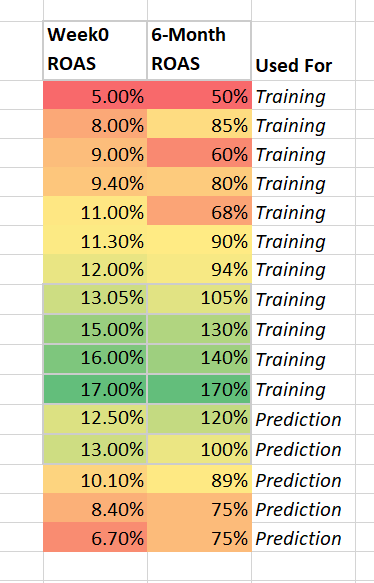
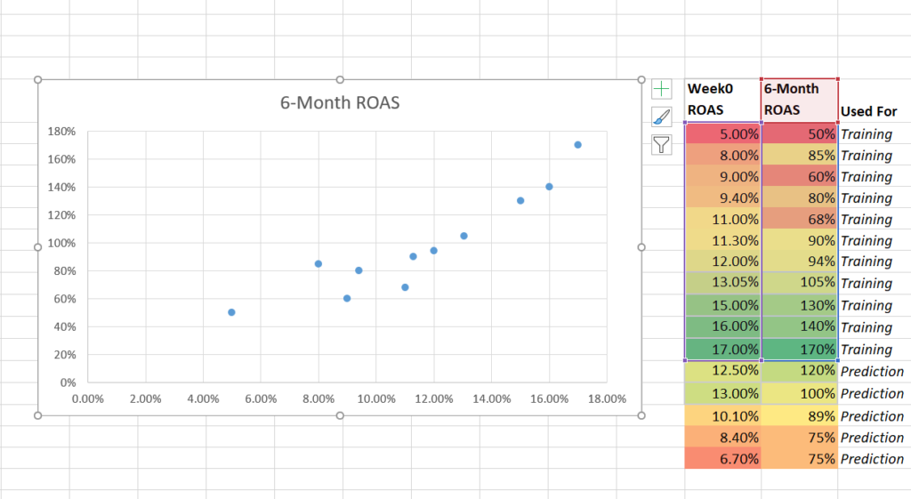
The first step to using Excel for predicting profit is to ensure you have enough Week 0 and 6-month data points. While you technically can draw a slope and make a prediction for any point on that slope with two data points, your prediction will be far from solid with so few observations powering it.
The ideal number of observations depends on a multitude of factors; such as your desired confidence level, correlations in the dataset, and time constraints, but as a rule of thumb for Week 0 ROAS-based predictions, you should shoot for at least 60 pairs of Week 0 and 6-month ROAS observations.
It’s also vital to include enough observations that have reached the goal level you set. If you have 60 data points to plot, but only 2 points where 6-month ROAS crossed 100%, then your equation model won’t be powered by enough of an understanding of what inputs are required to reach this breakeven point.
In this case, for all your model knows, the requirement to get to 100% ROAS after 6 months could be either another 2 full ROAS percentage points or 5 percentage points, which is a very wide range that is not conducive to predicting.
Step 2
Once you’ve gathered enough observations of the goal level, the second step is to split your data set into two groups, one for training and one for prediction.
Place the lion’s share of data (~80%) in the training group. Later on, you will use the prediction group to actually test your model’s accuracy of predicting the 6-month ROAS, given the Week 0 ROAS.
Step 3
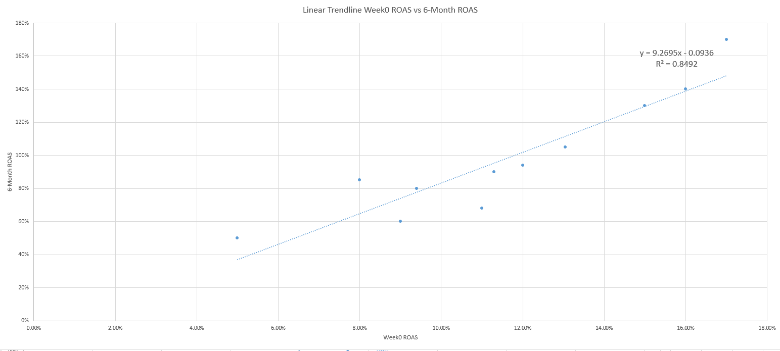
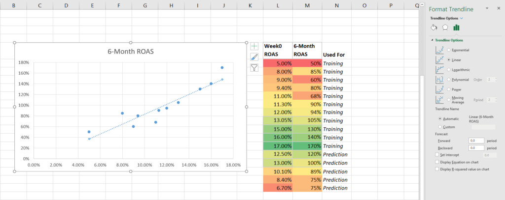
The third step is to use a scatter plot to graph the data, with Week 0 ROAS on the x-axis and 6-month ROAS on the y-axis.
Then add a trendline and add the equation and R-squared settings.
Graph the training data using a scatter plot.
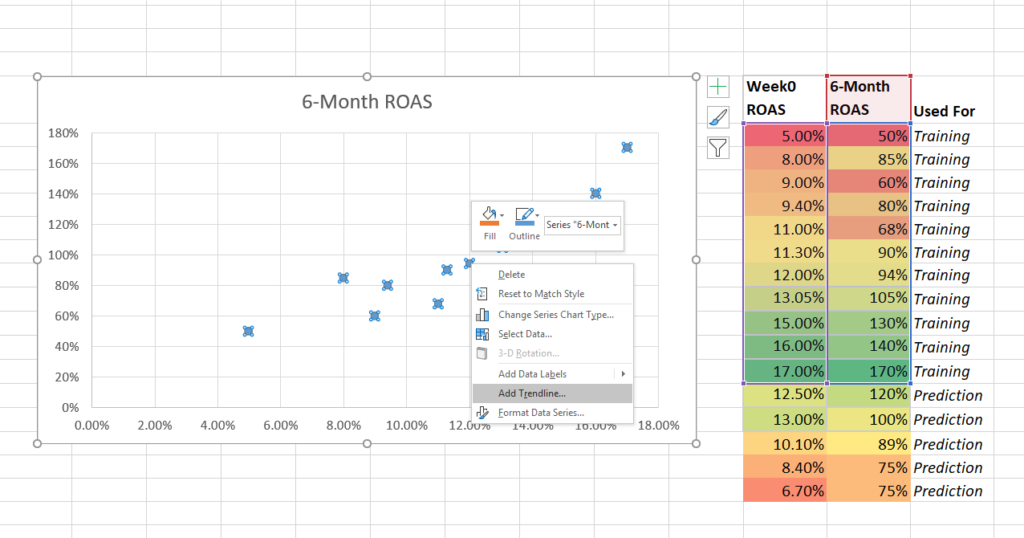
Right click on a data point and add a trendline.
Add the trendline equation and R-squared.
Step 4
Step four involves using the y = mx + b linear equation to solve the equation’s x value (Week 0 ROAS) when the y value (6-month ROAS) is 100%.
Rearranging the equation using algebra is done as follows:
1. y = 9.2695x – .0936
2. 1 = 9.2695x – .0936
3. 1 + .0936 = 9.2695x
4. 1.0936 = 9.269x
5. X = 1.0936 / 9.269
6. X = 11.8%
In this way, we calculate that the answer to the question of how to predict profit at 6-month – is that your ROAS must be greater than 11.8% in the first week.
If your Week 0 ROAS comes in under this rate, you know that you will need to adjust bids, creatives, or targeting to improve the cost / quality of your acquired users and improve your monetization trends.
If your Week 0 ROAS is over this number, then you can feel confident in raising budgets and bids!
Step 5
Step five is where you use your prediction segment of the full data set to assess how well your model was able to predict actual outcomes. This can be assessed using the Mean Absolute Percentage Error (MAPE), which is a calculation that divides the absolute value of the error (the actual value minus the predicted value) by the actual value.
The lower the sum of the MAPE, the better the predictive power of your model.
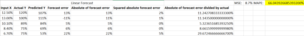
There is no rule of thumb for a good MAPE number, but generally, the more data your model has and the more correlated the data is, the better your model’s prediction power will be.
If your MAPE is high and the error rates are unacceptable, it may be necessary to use a more complex model. While more difficult to manage, models involving R and python) can increase the prediction power of your analysis.
And there you have it: a framework for predicting marketing campaign profitability.
But don’t stop reading yet! This guide has more goodness to come.
Improve your predictions
For the curious readers out there, the question on your mind may be whether the default, linear trendline is the best to use for predicting profit.
You may even try out a few more trendlines and discover that the R-squared (a measure of the fit of the equation to your data) improves with other equations, raising the profile of this question even more.
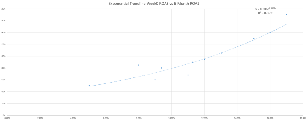
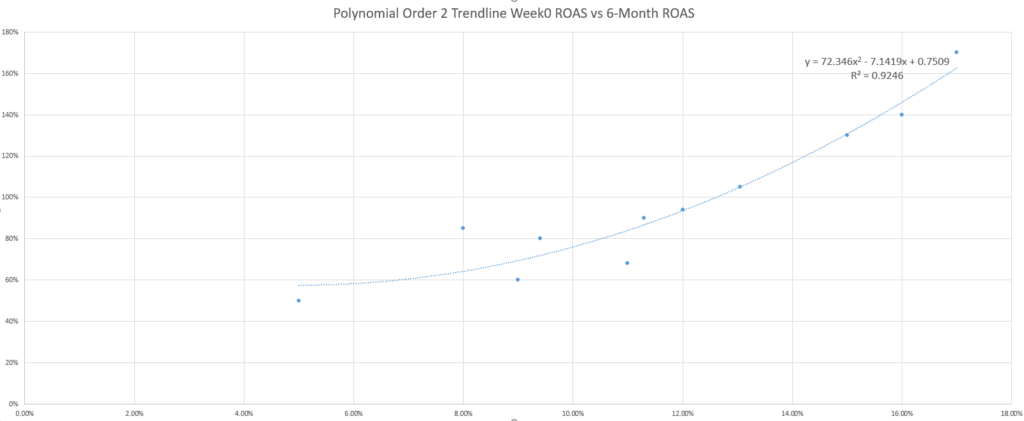
While the marketing adage of “it depends” applies again in selecting the best trendline, another marketing adage is useful as a response: KISS (keep it simple, stupid). If you are not a statistician or a math enthusiast, your best bet is to use the simpler trendlines – which is the linear one.
Why is this an issue? As a simple example, consider the addition of unexpected data into the model. In the following two scenarios, see how a lower Week 0 ROAS maturing unexpectedly well, or a higher Week 0 ROAS maturing unexpectedly poorly – affects each trendline model’s accuracy (assessed using the MAPE).
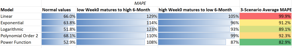
Using the MAPE to compare the different trendline-based models here shows that, while the linear and exponential models are not the most accurate in any case, they are the most consistent.
In addition, machine learning can give you the ability to automate this process, analyze greater amounts of data, and provide faster insights.
Making sure you’re going the right way
As a final note, check out this list of additional questions that can prove useful for ensuring your prediction analysis is formed on solid ground:
- Did you continue feeding your model to keep it trained on the most relevant data?
- Did you check to see whether your model’s predictions come to fruition based on new observations, or close to it?
- Do you have too much variation or, conversely, overfit?
- A very low R-squared or a very high R-squared are indicative of a problem in your model’s ability to predict new data accurately.
- Did you use the right KPI?
- Go ahead and test different KPIs (e.g. more or fewer days of ROAS or LTV) and use the MAPE to compare the profit prediction power of each.
You may be surprised at how poorly correlated the standard measures prove to be.
- Did your leading indicators or early benchmarks experience significant change?
- This can be a sign that something significant has shifted in the real world, and that trouble is brewing for your model’s ability to predict profit accurately moving forward.
- Did you apply segmentation to the data?
- Segmenting users into more homogenous groups is one great way to reduce noise and improve the predictive power of your model.
For example, don’t apply the same model to all users across all channels and geographies if those users have significantly different retention and cost trends.
- Are you considering the influences of time?
- Most marketers are aware of the influences of seasonality being a factor for which predictions can break down, but the lifecycle of your app/campaign/audience/creative can also influence the ability of your model to make accurate predictions.

Adding another piece to the puzzle: Predicting in-app ad LTV
In-app advertising (IAA) has become increasingly popular, accounting for at least 30% of app revenue in recent years. Hyper-casual and casual games, in addition to many utility apps, naturally leverage this revenue stream as their primary source of monetization.
Even developers who had been completely reliant on in-app purchases (IAP) have started monetizing with ads. As a result, we can see that many apps are now successfully combining both revenue streams to maximize their users’ LTV.
For example, look no further than King’s Candy Crush.
Hybrid monetization’s LTV is composed of two parts:
- In-app purchases/subscription LTV: Revenue actively generated by a user who purchases in-game or in-app currency, special items, extra services, or a paid subscription.
- In-app advertising LTV: Revenue passively generated by a user that views and/or interacts with ads (banners, videos, interstitials, etc.)
The data challenge
Ideally, marketers should be able to understand the nominal value of every single impression; that would practically make it a “purchase.” After gathering sufficient data, we’ll be able to create prediction models similar to what we’ve already described in chapter 2 for in-app purchases.
But in the real world, it’s not that simple – even calculating in-app ad LTV on its own is difficult because of the volume and structure of revenue data marketers are able to get their hands on.
To list a few issues:
- There’s rarely one source of ads that is being displayed. In reality, there are many, many sources, with an algorithm/tool behind them (ad mediation platforms) that constantly switch sources and eCPM.
- If one user views 10 ads, it’s quite possible that they came from 5 different sources, each with a completely different eCPM.
- Some ad networks pay for actions (install, click) rather than impressions, complicating things even further.
- When working with commonly used mediation platforms that offer user-level ad revenue, the number remains an estimate. The underlying ad networks often don’t share this data,usually leading to a division of generated revenue to users who viewed the impressions)
- eCPMs can drastically fluctuate over time and it is impossible to predict these changes.
In-app ad LTV prediction models
Many companies we interviewed were not actively involved with ad LTV predictions. Among gaming app marketers who were interested in the topic, none had this actually figured out to a level they’d be happy using it. Instead, it was more of a work in progress.
The following are the concepts that were discussed as transition points:
1. The retention-based/ARPDAU retention model
- Concept: Using the ARPDAU retention model, which in this case also contains the additional contribution of in-app ad revenue.
- Example: D1/D3/D7 retention is 50%/35%/25%. After fitting these data points to a power curve and calculating its integral until D90, we learn that the average number of active days is 5. Knowing that the ARPDAU is 50 cents, the predicted D90 LTV would therefore be $2.50.
2. The ratio-based method
- Concept: Integrating user-level ad revenue estimates into the stack in order to use the ratio method in the same way (i.e. based on coefficients from D1, D3, D7, etc).
- Example: ARPU calculated from both in-app purchases and in-app ad revenue is 40 cents after the first 3 days. We know that D90/D7 = 3. Predicted D90 LTV would therefore be $1.20.
3. The simple multiplication method
- Concept: Calculating the ratio between in-app purchases and ad revenue to use a multiplier for the total LTV calculation. With more data in place, multiple coefficients can be calculated for platform/country dimensions, as these usually have the biggest impact on the ad vs in-app revenue ratio.
Link to behavior-based LTV predictions
It’s important to mention another key factor that can heavily influence the potential profitability of app users: cannibalization.
Users spending money by making in-app purchases often have a significantly higher LTV than users that just consume ads. It’s of the utmost importance that their intent is not disrupted by free handy stuff messages.
On the other hand, it’s important to incentivize users to watch ads, so they’re often rewarded with in-app currency or bonuses.
If an app contains both rewarded ads and in-app purchases, it is possible that, at a certain point, a player that would otherwise become an IAP spender would not due to a significant reward of in-app currency in return for watching ads.
This is exactly where behavioral predictions come into play — by measuring users’ behavior, a machine learning algorithm can determine the likelihood that certain users would become “spenders” and indicate where certain tweaking of game/app experience is required.
The process works as follows:
- All users should start with a no-ad experience while engagement data begins to be measured.
- The algorithm continuously calculates a probability of a user becoming a spender.
- If this probability is over a set percentage, ads will no longer be shown as more data is gathered (“waiting for the purchase”).
- If the probability falls below a set percentage, it’s most likely that this user will never make a purchase. In this case, the app starts showing ads.
- Based on players’ longer-term behavior, the algorithm can continue evaluating their behavior while modifying the number of ads and mixing up between different formats.
Most companies will be content with using simple models and approaches that will deliver the optimal cost/benefit ratio, specifically when it comes to implementation difficulties and the added value of more precise insights.
Rapid advances in this area can already be seen, with different solutions coming in to fill the gaps and complement the ecosystem’s frantic development pace, as well as the growing importance of in-app advertising as a key revenue stream for apps.
The contribution method
While well-tuned behavior prediction methods may yield the most accurate results in attributing ad revenue, there is a simpler and more viable method for handling the issue of assigning ad revenue to an acquisition source.
This method is based on allocating a channel’s contribution of ad revenue according to aggregated user behavior data points.
Contribution margins work by converting a channel’s contribution to overall user behavior – into that channel’s earning margin from the overall ad revenue generated by all users.
The theory is that the more a channel’s acquired users generate actions in an app, the more influential and deserving that channel’s hand in claiming credit for advertising revenues from those users.
To clarify, let’s break it down:
Step 1
The first step involves selecting a data point to use for determining each acquisition source’s ad revenue contribution margin.
As a starting point, you can use Excel trendline regression to identify which user behavior KPI best correlates most with changes in advertising revenue.
Note that, because the contribution method involves attributing revenue based on a proportion of total activity, you will want to use a data point that is a count-like number of active users in a day, rather than a ratio-like retention rate.
A few options include:
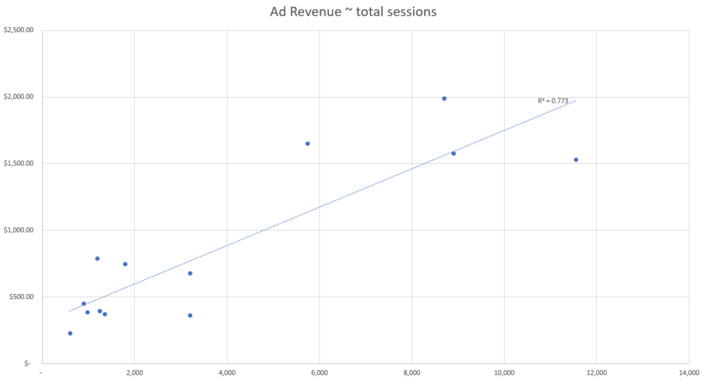
- Total active users
- Total user sessions
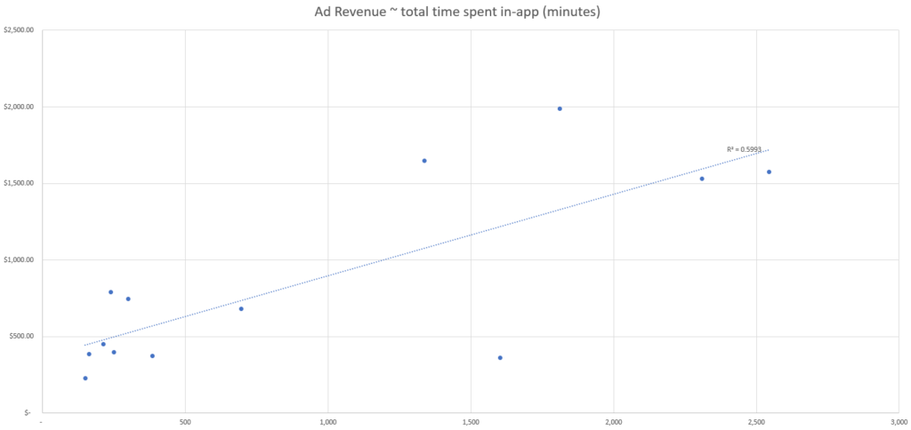
- Total session duration
- Ad-attributable data (e.g. ad impressions)
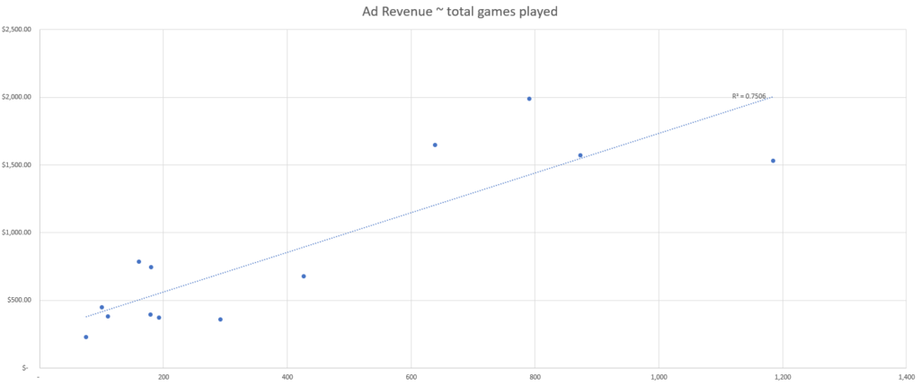
- Total key events (e.g. games played)
Step 2
Once you have a few data points to observe, scatter plot each data point against total ad revenue per day in order to see where the correlations between changes in user behavior and total ad revenue are strongest.
Step 3
Add the R-squared data point to your graph to identify which data point has the strongest correlation.
There is one downside to this Excel trendline regression method: the less variation in user behavior and ad revenue, the less accurate the model’s ability to observe the strength of correlation between data points.
As a result, you will have less confidence in being able to choose one data point over another.
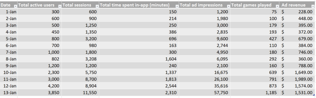
In this simulated dataset, we see the counts of each data point, per day, as well as the total ad revenue generated per day.
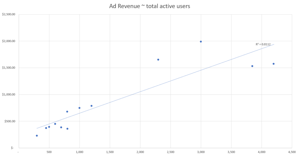
Based on this simulated data, we can see that the event with the best correlation strength appears to be the number of active users based on our R-squared fit metric.
This means that the data point from our set which best explains changes in ad revenue is the number of active users, and therefore we should use the number of active users to attribute ad revenue by channel.
Step 4
Once you have selected a user behavior KPI, it’s time to calculate the contribution margin.
Then, multiply each channel’s daily contribution margin by the cumulative ad revenue generated on each day.
This process requires that the user behavior data be measured per channel and accessible every day, so that the contribution margin of all channels can be calculated with each new day’s revenue data.
Note: while we only include four ad channels here for illustrative purposes, you might also want to include your organic and other channel data here, in order to fully attribute the daily revenue to daily user behavior.
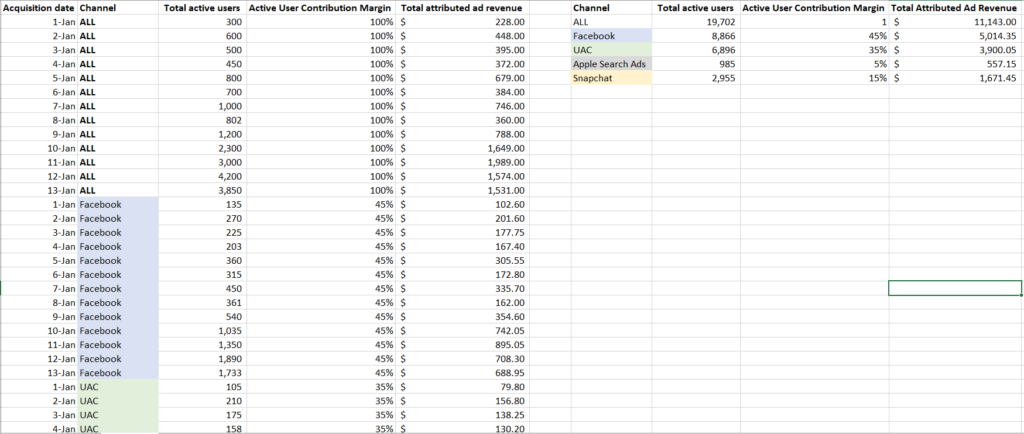
Above, we can see the calculated ad revenue generated by day, by channel, which allows you to estimate the profitability of each channel.
Note that you will need to revisit your assessment of useful KPIs for ad revenue attribution as user behavior trends and ad revenue monetization data shift, or as new data points become available.
For example, in the above dataset, we can see a second grouping of data points towards the end of the data period (starting roughly January 10th), where there is significantly more ad revenue per day than earlier in the month.
This is reflected in the grouping of data towards the top-right of each scatterplot, away from the bottom-left group.
The more complex the dataset, the less accurate this simple Excel regression assessment will be, and the greater the need to apply segmentation and a more rigorous analysis.

Predictive modeling in a privacy centric reality
Heading into a new advertising reality
Predictive analytics allows you to increase your campaign’s potential audience, drive higher user LTV, and ensure more efficient budgeting – in an era where in some cases we no longer have access to granular performance data.
By creating different behavioral characteristic clusters, your audience can then be categorized not by their actual identity, but by their interaction with your funnel in its earliest stages. This interaction can indicate their future potential to drive meaningful value to your product.
Combining key engagement, retention, and monetization factors can correlate to a user’s compatibility with any developer’s LTV logic, and provide a pLTV (Predicted Lifetime Value) indication at the very beginning of a campaign.
Machine learning – key to success
A mobile app may have 200+ metrics available for measurement, but a typical marketer will probably only measure a maximum of 25. A machine, on the other hand, is able to ingest all of that information in a matter of milliseconds and apply it to marketing insights and app functionality indicators.
A machine learning algorithm will be able to calculate all these indicators and find the right correlations for you. Its calculations will be based on your definition of success, your LTV logic, and apply that to a significant amount of data to find correlation between early engagement signals and eventual success.
This means that advertisers no longer need to know WHO the user is, but rather know WHAT pLTV profile and characteristics they fit into. This profile should be as accurate as possible, and made available during the campaign’s earliest days. It should represent the advertiser’s LTV requirements for it to be considered valid and actionable.
When it comes to eCommerce apps, for example, applying indicators such as previous purchases, frequency of purchases, time of day, or funnel progression allows the algorithm to cluster general audiences into highly granular, mutually exclusive cohorts.
This enables more effective targeting and messaging, and ultimately a higher ROAS.
Leveraging cluster LTV predictions
Predictive analytics help to cut the campaign learning period by using existing integrations to provide an accurate campaign LTV prediction.
By leveraging machine learning and understanding aggregated data, predictive analytics could feasibly deliver a campaign potential indication in the form of a score, ranking or any other form of actionable insight within days of its launch, informing marketers how successful it is likely to be.
For example, a gaming app’s machines found that users who complete level 10 of a game within the first 24 hours are 50% more likely to become paying users.
With this information, marketers can either cut their losses on a bad campaign that doesn’t deliver quality users, optimize where required, or double down when early indications show potential profit, giving them the ability to make fast pause-boost-optimize decisions.
The SKAdNetwork challenge
The introduction of iOS 14’s privacy-focused reality and Apple’s SKAdNetwork has created its own set of challenges, primarily limiting the measurement of user-level data in the iOS ecosystem to consenting users.
This is considered to be merely the first step towards a more user privacy-focused advertising environment, with many of the online industry’s biggest players likely to follow in one form or another.
These changes limit not only the volume of available data, but also the time window in which marketers can make informed decisions on whether a campaign is likely to be successful or not.
Although machine learning algorithms can quickly predict which campaigns are likely to deliver the most valuable customers, other limitations include a lack of real-time data, no ROI or LTV data as it mostly measures installs, and a lack of granularity as only campaign-level data is available.
So how can you deliver relevant advertising without knowing what actions each user is performing?
You guessed it: Machine learning-powered predictive marketing. Using advanced statistical correlations based on historic app behavior data to predict future actions, marketers can run experiments using non-personalized parameters, such as the contextual signals and continuous machine learning models training.
The results can then be applied to future campaigns and further refined as more data is collected.

Best practices for building mobile marketing prediction models
1. Feed the beast
When building data models that are used to guide significant decisions, it’s not only important to build the best system possible, but also to perform ongoing testing to ensure its effectiveness.
For both purposes, make sure that you continuously feed your profit prediction model to keep it trained on the most relevant data.
In addition, always check whether your model’s predictions come to fruition based on new observations, or at least close to it.
Not following these steps could mean that a model with an initial useful prediction power could go off the rails depending on seasonality, macro auction dynamics, your app’s monetization trends, or many other reasons.
By observing your leading indicators or early benchmarks and looking for significant changes in data points, you can gauge when your own predictions are likely to break down, too.
For example, if your model was trained on data where the average day 1 retention rate ranged from 40%-50%, but for the stretch of a week, the day 1 retention rate dropped to 30%-40%, this could indicate a need to re-train your model.
That might be especially true given that quality signals from the users you most recently acquired have shifted, likely leading to changes in monetization and profit, all else equal.
2. Choose the right KPI for predicting profitability
There are several options to choose from, each with a set of trade-offs in viability, accuracy, and speed to produce recommendations.
Go ahead and test different KPIs (e.g. more or fewer days of ROAS or LTV) and use one or all of the following to compare the profit prediction power of several KPIs:
- R-squared
- A ratio of success-to-failure at satisfactory predicting
- Mean Absolute Percentage Error (MAPE)
You may be surprised at how poorly correlated the standard measures prove to be.
3. Segment your data
Segmenting users into more homogenous groups is not only a great way to improve conversion rate, but also a proven method to reduce noise and improve the predictive power of your model.
For example, applying the same model to both interest-based campaigns and value-based lookalike campaigns could lead to less effective results. The reason for this is that monetization and length of lifetime trends of users from each unique audience target are likely to be significantly different.
Additionally, by creating different behavioral characteristic clusters, your audience can then be categorized not by their actual identity, but by their interaction with your campaign in its earliest stages. This interaction can indicate their future potential with your product.
For example, a gaming app developer can predict the potential LTV they can drive out of their users in a 30-day time frame. In other words, the period of time until a tutorial completion (engagement), number of returns to the app (retention), or the level of exposure to ads across each session (monetization).
4. Remember to factor time
Most marketers are aware of the influences of seasonality on breaking down predictions, but the lifecycle of your app/campaign/audience/creative can also influence the ability of your model to make accurate predictions.
The acquisition cost trends in the first week of a new app launch will be much different from those in the fifth month, the second year, and so on, just as the first 1,000 dollars in spend in a previously untapped lookalike will be different than the 10,000 and 50,000 dollar in spend invested into the same lookalike (especially without changing the creative used).

Key takeaways
- The science of predictive analytics has been around for years, and used by the biggest companies in the world to perfect their operations, anticipate supply and demand shifts, foresee global changes, and use historical data to anticipate and prepare for future events.
- As we head into a new, privacy-centric reality we must adopt a new measurement standard – one that requires shorter measurement time frames and applies anonymous user potential indications for decision making.
- Predictive modeling does just that. Introducing this sophisticated technology to the marketing landscape and its application to accommodate the industry’s evolution – is nothing short of paramount.